The random walk method on the space of unit quaternions produces uniformly distributed quaternions without trigonometric functions. We study some performance and quality properties. Implementations in SIMD and GLSL are provided.
1. Quaternions as rotations
Consider the space of quaternions
where
By linearity, these rules define a multiplication among quaternions. Using the norm of
Since for two quaternions
Note that
This isomorphism lets us understand how quaternions act on two complex planes
The common algorithm1 for producing random quaternions using these planes is
quat rand_quat()
{
	float phi   = rand_float(0,2*pi);
	float theta = rand_float(0,2*pi);

	float z = rand_float(0,1);
	float r = sqrt(z);
	float t = sqrt(1.f-z);
	return {r*cos(phi), r*sin(phi), t*cos(theta), t*sin(theta)};
}
We shall refer to this algorithm (and its variations) to either the polar method or Marsaglia’s algorithm.
Quaternions are useful because of the two-to-one representation
which are the images of
Identify
With respect to this basis
which is the usual formula given to convert a quaternion into a rotation.2
It is useful to have a complete multiplication rule in terms of the scalar real and the 3-dimensional imaginary part of a quaternion: Let
where the angle brackets denote the 3-dimensional inner product and the multiplication sign denotes the cross product. If
Substitute
This results in commonly known GLSL code for quaternion-vector multiplication.4
vec3 quat_mult(vec4 q, vec3 v)
{
   return v + 2*cross(q.yzw, (q.x*v + cross(q.yzw, v));
}
2. Random quaternions
Our goal is to produce a random unit quaternion or a random rotation
Up to normalization, it is the unique translation invariant measure: For any6 subset
Equivalently, we can use the uniform measure
Algorithms which produce random rotations are discussed in the Graphics Gems series,7 II and III by Arvo and Shoemake.8 These include the Box-Muller method to first produce a Gaussian random variable in 4 dimensions. Since it is rotation invariant, all is left is to normalize. The other proposed method is the subgroup algorithm where the fact is used that
We note that the rejection method in which we sample the 4-dimensional cube
3. Integer quaternions and the tree structure
Quaternions already make sense over the integers,12 and a fundamental fact for the method discussed in this post.
The group
The following quaternions give rise to a free group of rank 3 inside
If we want to write them as unit quaternions, we have to divide by their norm
The associated rotations are
and their inverses. In fact, for any prime
and
A proof that these generate free groups can be found in Lubotzky’s book.14
4. Random walk
The simple random walk on the graph generated by
starting at the identity element which is the root of the tree
Here is a pseudo C++ implementation:
float s5 = 1.f/sqrt(5.f);
quat s[6]
{ 			s5*quat{1, 2,0,0},
			s5*quat{1,0, 2,0},
			s5*quat{1,0,0, 2},
			s5*quat{1,-2,0,0},
			s5*quat{1,0,-2,0},
			s5*quat{1,0,0,-2},
};

mat3 random_rotation(quat &state)
{
   u32 a = uniform_int(0,5);        // Draw an integer in [0,5].
   state = quat_mult(s[a], state);  // Update the internal state q.
   return rot_from_quat(state);     // Return the rotation matrix R_q.
}
5. Convolution and spectral gap
It was shown by Lubotzky, Phillips and Sarnak15 (LPS) that the convolution operator associated to these elements has the strongest possible spectral gap possible.
To explain what this means, we pick out the tree
LPS show that if we consider the average operator
Here one restricts to functions orthogonal to the constant function
The
Thus, there exists
From here one can also deduce a discrepancy result: Let
equivalently, the sphere of radius
There exist some exponent
The theorems of LPS show that the balls and spheres in tree
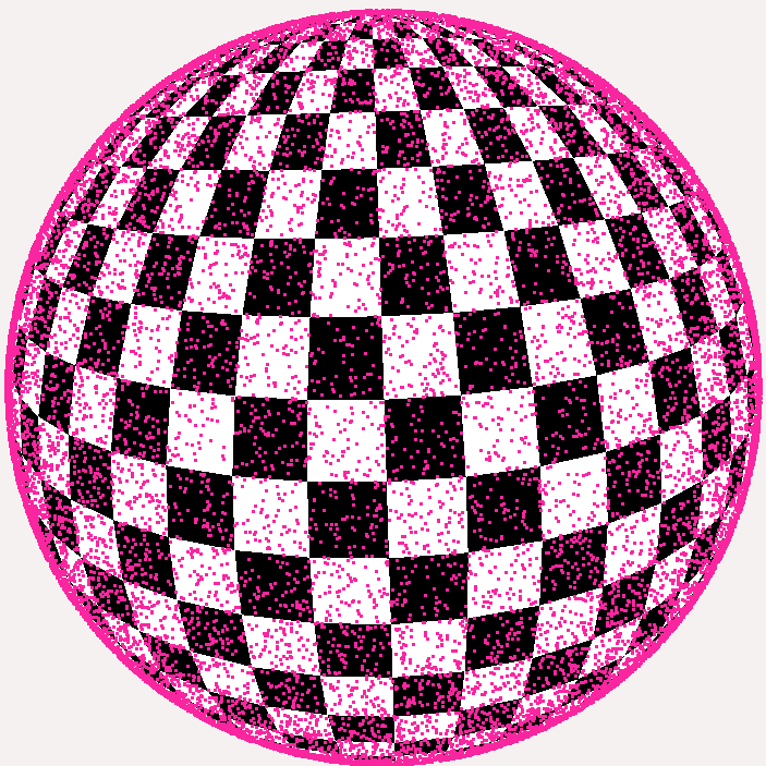
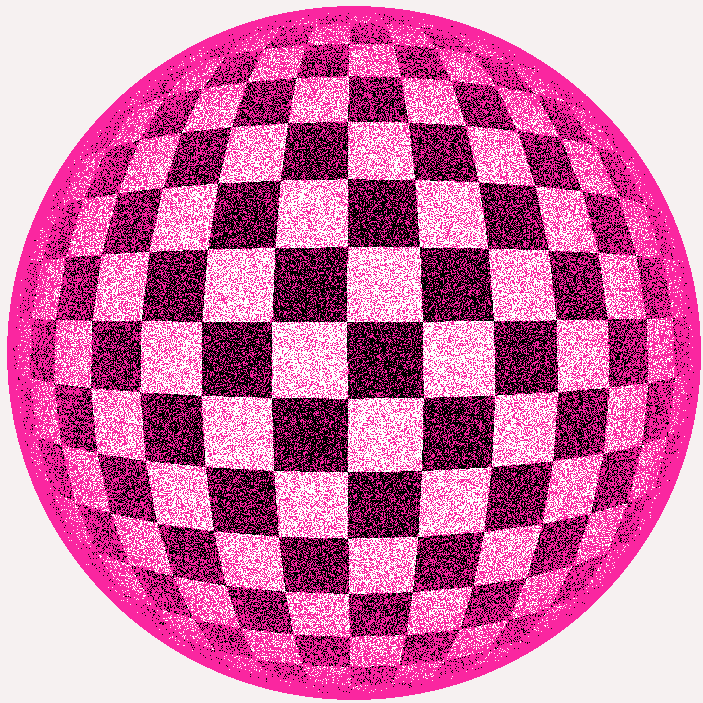
Here are images of the spheres of radius 5, 6, and the whole tree up to radius 8.
For each quaternion, we plotted three points, the images of the rotation action under the standard basis.
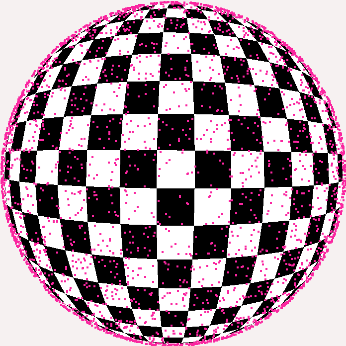
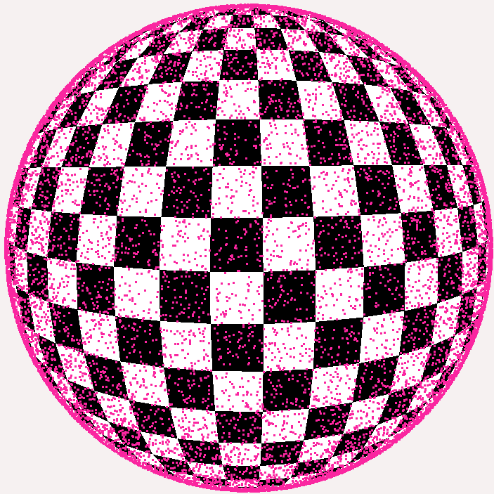
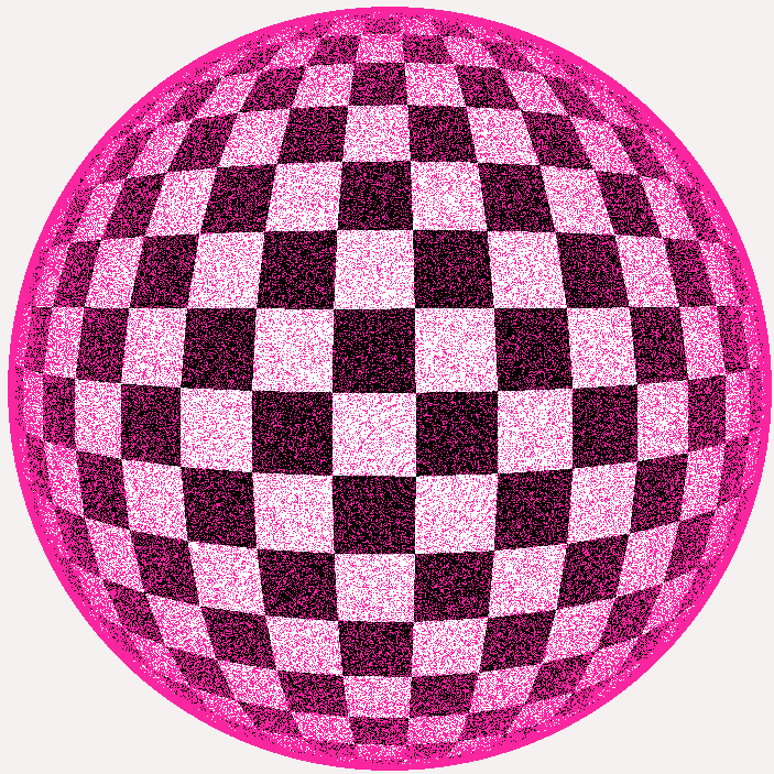
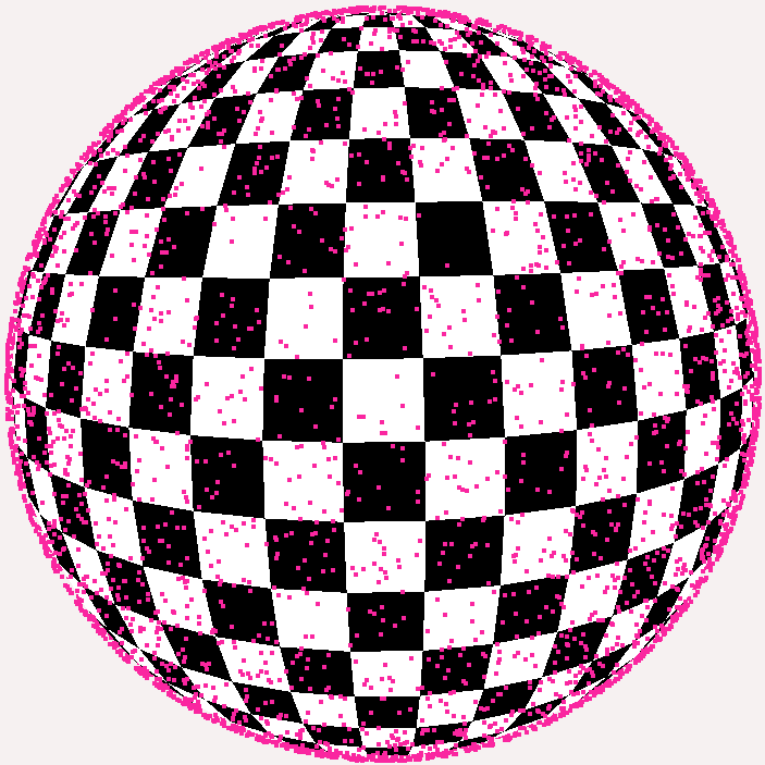
For comparison, here is the polar method for the same number of points:
6. Nonbacktracking random walks
The dynamics related to
For the next move, we restrict to
The non-backtracking walk will have to save the last step in its internal state. Using the particular ordering in the array, if the last step was
struct internal_state { quat q; u32 last_choice; };
mat3 random_rotation_nonbacktracking(internal_state &state)
{
   u32 a = ( state.last_choice + 4 +  uniform_int(0,4)) % 6;
   state.q = quat_mult(s[a], state.q);
   state.last_choice = a;
   return rot_from_quat(state.q);
}
We omitted the seed for the uniform integer generator which should also be part of the internal_state struct.
7. Equidistribution of the the random walk
As suggested more recently,18 the spectral gap of the operator
The large deviation principle states that the fraction of walks
decays exponentially as
The law of large numbers (LLN) can be phrased as follows:
Let
We wish to show the law of large numbers for sum of random variables
where
or uniformly among
For brevity, we restrict now to the simple random walk.
Let
The space of all paths is
The expectation
Applying the above operator bound from the spectral gap discussion,
since the error term sum to a geometric series bounded by a constant.
Analogously one shows that the variance behaves like
using that if
The pointwise convergence of
It follows from Breiman’s LLT for Markov chains,19 which applies to both the simple random walk and the non-back tracking walk, that
Using these bounds it is also possible to deduce a central limit theorem.20
8. Estimating the discrepancy
The results in LPS refer to the following setup.
Pick a point
In LPS, the spherical cap discrepancy is employed. A spherical cap is determined by a unit vector
Given a point set
An analytically easier discrepancy is the mean square spherical cap discrepancy
where
LPS prove
The exponent
LPS also did numerical experiments in Pascal. They formulated the results in terms of the error exponent,
The rotations associated to
More recently, in a study on illumination integrals21 the Stolarsky’s invariance principle22 has been employed to measure discrepancy for point sets on the 2-sphere. Consider the following expression
which sums the distances within the point set. Then the principle states
which gives a trivial way to measure discrepancy for moderately large sets for which an
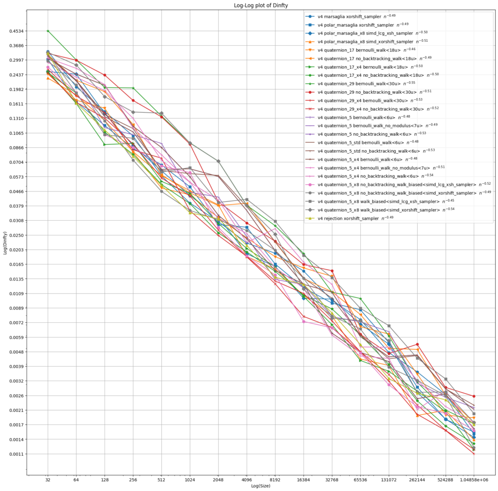
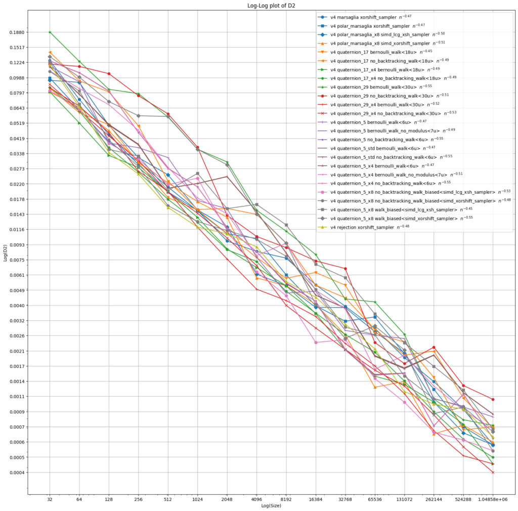
While the energy method works well for small n, we employ Monte Carlo integration to calculate the defining integral of the mean square integral (which involves integral over the 4-sphere). We employ the Super-Fibonacci Spirals23, which is the state-of-the-art method for low discrepancy quaternions if n is known in advance. The discrepancy of that point set is an order of magnitude lower compared to the discrepancies of the random methods studied here.
The following plots show the extremal and mean square spherical discrepancy for up to a million points. Points are produced using various primes p, various integer random number generators and various random walk laws. Some of these will only be discussed later. We observe an error exponent of around 0.5 for all these variations.
9. Biased walks to avoid modular arithmetic
It is also possible to obtain equidistribution if the law for the choice among
quat s5_biased[8]
{ 			s5*quat{1, 2,0,0},
			s5*quat{1,0, 2,0},
			s5*quat{1,0,0, 2},
			s5*quat{1,-2,0,0},
			s5*quat{1,0,-2,0},
			s5*quat{1,0,0,-2},
                        s5*quat{1, 2,0,0},
                        s5*quat{1,0, 2,0},
};

mat3 random_rotation_biased(quat &state){
   u32 a = random_int() & 7;        // Draw an integer in [0,7].
   state = quat_mult(s5_biased[a], state);
   return rot_from_quat(state);
}
10. Performance and SIMD implementation
A quaternion fits into a 128-bit SIMD register:
union mm_quat
{
	__m128 mm_q;
	quat q;
};
Quaternion multiplication in compressed SIMD accumulates to around a dozen SSE instructions.26 Quaternion to rotation matrix (and back) is discussed by van Waveren27 and available in the Doom 3 BFG Edition GPL source code.28 In this approach, we can still use the previous implementation for advancing the random walk.
We measure performance on two tests, “write” and “sample”. In the write test we simply fill a large array of quaternions. The sample test not only produces quaternions but immediately uses them to calculate the discrepancy. We produce
On a AMD Ryzen Zen 4 we count around 14 cycles per write and 100 cycles per sample for the scalar versions. A look at the disassembly shows that the MSVC compiler uses 128-bit SIMD. Marsaglia’s algorithm is implemented both using the rejection algorithm and the polar algorithm for sampling on a disk with a cycle count of 50/100 for write and 70/110 for sample.
The custom SIMD by compression is profiled with 20 cycles resp. 40 cycles.
In contrast, we can employ SIMD instructions by optimizing for throughput, here the 256-bit variant:
struct quatx8
{
	__m256 r,x,y,z;
	quatx8() : r(_mm256_set1_ps(1.)), x(_mm256_set1_ps(0.)),
                   y(_mm256_set1_ps(0.)), z(_mm256_set1_ps(0.)) {}
};
Multiplication and the transform to a rotation matrix is a straight forward translation from the corresponding scalar code. The write test will additional have a struct-of-arrays to arrays-of-struct routine that will shuffle quatx8 to quat[8].
Instead of using an array, we construct the elements of __m256 variables in-place using the following function construct_T5.
// Encode each element in three bits: s_i = b2b1b0
//b0 = sign.
//b2b1 in {0,1,2,3} where 2 and 3 both get mapped to choice 2
quatx8 construct_T5(__m256i s)
{
   const __m256 s5_x8 =_mm256_set1_ps(1./std::sqrt(5.));
   const __m256 s5_2_x8 =_mm256_add_ps(s5_x8,s5_x8);
   const __m256i one = _mm256_set1_epi32(1);

   __m256 a = _mm256_xor_ps(s5_2_x8, _mm256_castsi256_ps(_mm256_slli_epi32(s,31))) ;
   s = _mm256_srli_epi32(s, 1);
   __m256 x = _mm256_and_ps(a, _mm256_castsi256_ps(_mm256_cmpeq_epi32(s,
                                                         _mm256_setzero_si256())));   // == 0?
   __m256 y = _mm256_and_ps(a, _mm256_castsi256_ps(_mm256_cmpeq_epi32(s,one)));   // == 1?
   s = _mm256_srli_epi32(s, 1);
   __m256 z = _mm256_and_ps(a, _mm256_castsi256_ps(_mm256_cmpeq_epi32(s,one)));   // >= 2?

   return { s5_x8, x, y, z };
}
While the biased simple random walk is straight forward to translate, we come up with a new scalar version for the non-backtracking random walk avoiding modulus which is missing in AVX2.
We reorder the array as to have the pair
Then we set (arbitrarily) the rule that if we were to walk back, we instead repeat the previous choice, that is, walk forward in the same direction.
struct no_backtracking_walk_scalar
{
	u32 seed;
	u32 last;
};

u32 random_int(u32 seed);

u32 step(no_backtracking_walk_scalar *walk)
{
   u32 x = rng(walk->seed) & 7;
   x = x > 5 ? x-2 : x;  // The last two choices are copies.
   const u32 forbidden = walk->last & 1 ? walk->last-1 : walk->last+1;
   walk->last = forbidden == x ? walk->last : x;
   return walk->last;
}
Note that there are now two sources of bias. The first is the same from the “no integer arithmetic” optimization where we fill up the array to be of size 8.
But this time, we also wish to keep the non-backtracking property, so if we were to backtrack, we walk forward in the same direction instead. Effectively, this makes repeating the last step twice as likely. The convergence of the associated Markov chain is likely to hold.29
The AVX version could look something like this:
struct no_backtracking_walk
{
   __m256i seed;
   __m256i last;
};

__m256i step(no_backtracking_walk *walk)
{
   const __m256i one =_mm256_set1_epi32(1);
   const __m256i two =_mm256_add_epi32(one,one);
   const __m256i five = _mm256_set1_epi32(5);
   const __m256i seven= _mm256_add_epi32(two,five);

   const __m256i sign_bit = _mm256_and_si256(walk->last, one);
   const __m256i sign_bit_h = _mm256_cmpeq_epi32(sign_bit, one);
   const __m256i forbidden  = _mm256_blendv_epi8(
                              _mm256_add_epi32(walk->last, one),
                              _mm256_sub_epi32(walk->last, one),
                              sign_bit_h); // flip lsb which encodes sign

   __m256i x = _mm256_and_si256(rng(walk->seed), seven);
   const __m256i too_big = _mm256_cmpgt_epi32(x, five);
   x = _mm256_blendv_epi8(x, _mm256_sub_epi32(x, two), too_big);
   const __m256i is_backtracking = _mm256_cmpeq_epi32(x, forbidden);
   walk->last = _mm256_blendv_epi8(x, walk->last, is_backtracking);
   return walk->last;
}
The biased simple random walk flies through with 2 cycles per write and 7 cycles per sample. The write is three times faster than Marsaglia’s algorithm when implemented using the Intel math SSE library for sincos whereas the sample test gives comparable results.
The following plots summarize the data. They also include the discrepancy for the produced set of 65536 quaternions.
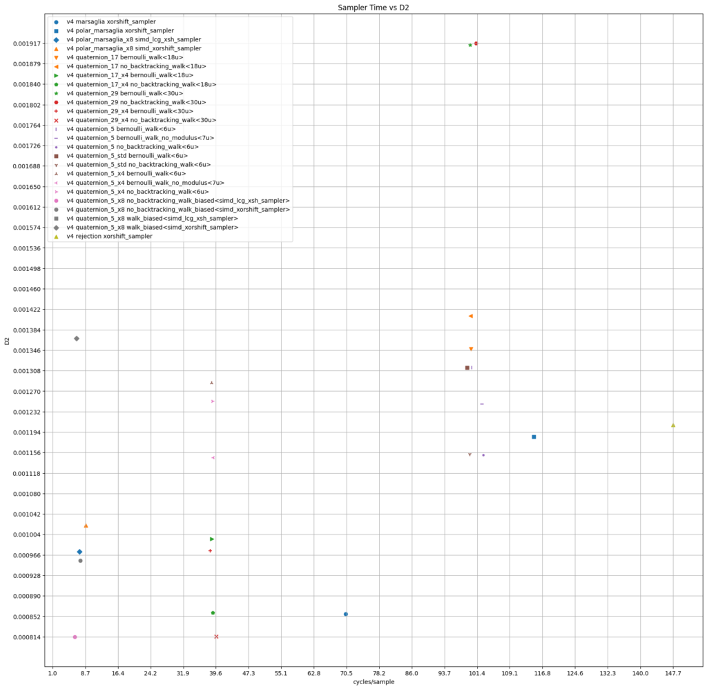
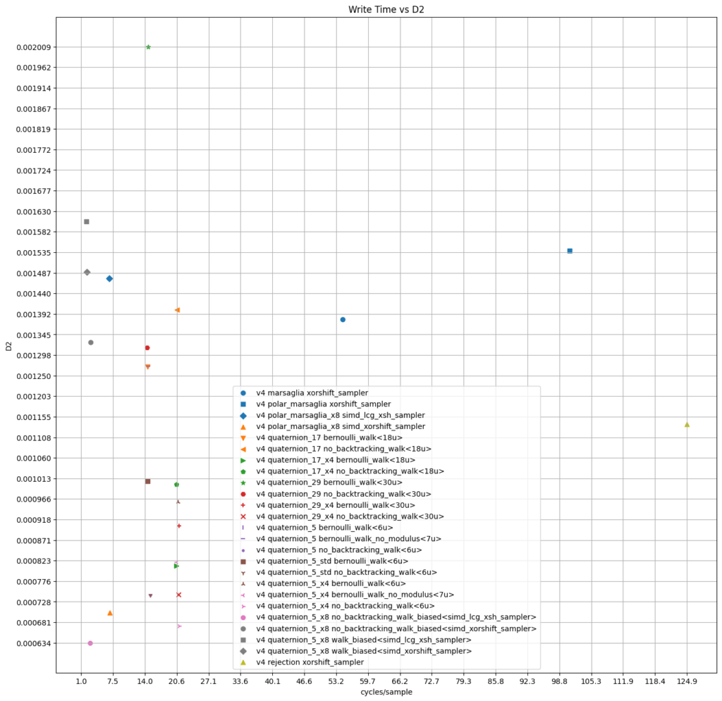
11. GLSL implementation
For the following we set our task to generate one or more quaternions per pixel per frame for some fictional graphical application.
A compute shader is run for every frame and each kernel invocation accounts for a pixel.
A seed is generated from the pixel location
The set of quaternions for a fixed frame
The generated sets for different frames should differ.
Here we chose to measure the time that it takes to calculate the discrepancy of the quaternions produced in each frame. We produce 1024 quaternions per frame, that is, have a loop of length 1024 in each compute invocation.
There is not a straight forward implementation of the random walk method without an explicit formula for the nth word given a list of choices (other then naive multiplication). Further, random walks of short length starting at the same position will produce the same elements.
To accommodate this difficulty, we first produce
random elements among
Here we use
vec4 quat_mul(vec4 a, vec4 b)
{
	return vec4(a.x*b.x   - dot(a.yzw, b.yzw),
                   a.x*b.yzw + b.x*a.yzw + cross(a.yzw, b.yzw));
}

#define s5inv   0.4472135f
#define s5inv2  0.8944271f
vec4 construct_ts(uint u)
{
	u = u & 7;
	float r = s5inv - (u&1u)*s5inv2;
	u >>=1;
	float x = u==0 ? s5inv2 : 0;
	float y = u==1 ? s5inv2 : 0;
	float z = u>=2 ? s5inv2 : 0;
	return vec4(r, x , y, z);
}

const uint shared_size = 1024;
shared vec4 tree_root[shared_size];

void rand_quat_init()
{
        uint id = gl_LocalInvocationIndex;
	uint id5 = id/5;
	uint id25 = id5/5;
	uint id125 = id25/5;

	tree_root[id] =  id < 750 ? vec4(1,0,0,0) : construct_ts(0);

	uint cur = id125;
	tree_root[id] = quat_mul( construct_ts(cur % 6) , tree_root[id]);
	memoryBarrierShared(); barrier();

	cur = cur+ 4 + id25 % 5;
	tree_root[id] = quat_mul(construct_ts(cur % 6) , tree_root[id]);
	memoryBarrierShared(); barrier();

	cur = cur + 4 + id5 % 5;
	tree_root[id] = quat_mul(construct_ts(cur % 6), tree_root[id]);
	memoryBarrierShared(); barrier();

	cur = cur + 4 + id % 5;
	tree_root[id] = quat_mul(construct_ts(cur % 6), tree_root[id]);
	memoryBarrierShared(); barrier();
}

vec4 rand_quat(uvec4 seed)
{
	seed = pcg4d(seed);
	vec4 p = quat_mul( tree_root[ seed.y  & shared_size-1], tree_root[seed.x & shared_size-1]);
        return p;
}
In each loop iteration, we can either multiply with random point on the larger sphere stored in shared memory (“random_walk_s5_4”) or go through it iteratively (“sphere_walk_s5_4”).
// Loop over 0<=i<1024

case random_walk_s5_4:
	{
	seed.x = pcg(seed.x);
	q = quat_mul( tree_root[seed.x & shared_size-1], q);
	break;
        }
case sphere_walk_s5_4:
	{
	q = quat_mul( tree_root[i & shared_size-1], q);
	break;
	}
We compare these algorithms to the polar version of Marsaglias algorithm, the Super-Fibonacci algorithm, and the non-uniform rejection algorithm which samples in the 4-cube and normalizes to one.
Here is a table for the throughput and discrepancies on a Nvidia RTX 4700 for creating 16’777’216 quaternions per frame for 1000 frames in total. “GSample” is measures the number of intersections (in billions) for the discrepancy test per second. The number of intersections is equal to the number of quaternions produced times the number of quaternions used in the Monte Carlo integration (here 512 or 1024 via the Fibonacci method).
Operations from the sum redux in each compute shader invocation to calculate the discrepancy are not measured.
For reference, according to the hardware specification30 the theoretical peak performance is 29 TFlops.
We also measure performance for the integrated GPU of a AMD Zen 4 Ryzen CPU on a smaller point set. The compute experiments are run both in OpenGL & GLSL and with Vulkan & GLSL/SPIR-V. The Vulkan program is used to be able to switch between the discrete and integrated GPU. For the discrete GPU, the OpenGL and Vulkan versions give similar results (though the shader compilation differs).
Numbers in parenthesis refer to the standard deviation.
| Nvidia RTX 4700 | n=16’777’216 | Zen 4 Ryzen integrated GPU | n=2’097’152 | |
| Algorithm | GSample mean/stddev | Discrepancy mean/stddev | GSample mean/stddev | Discrepancy mean/stddev |
| Sphere Walk S5_4 | 4045 (49) | 0.000107 (0.000008) | 88 (0.03) | 0.000347 (0.000080) |
| Random Walk S5_4 | 3167 (32) | 0.000125 (0.000016) | 67 (0.02) | 0.000308 (0.000048) |
| Marsaglia PCG | 2971 (32) | 0.000104 (0.000020) | 43 (0.01) | 0.000316 (0.000062) |
| Marsaglia PCG3 | 3295 (33) | 0.000103 (0.000020) | 41 (0.01) | 0.000304 (0.000059) |
| Super-Fibonacci | 3167(32) | 0.000009 (0) | 68 (0.02) | 0.000037 (0) |
| Non-uniform Rejection | 3126 (31) | 0.009137 (0.000010) | 38 (0.01) | 0.009007 (0.000019) |
The next plot shows the distribution of discrepancy for various seeds (i.e. for different frames). To decipher the axis, it is best to open the image it in a new tab.
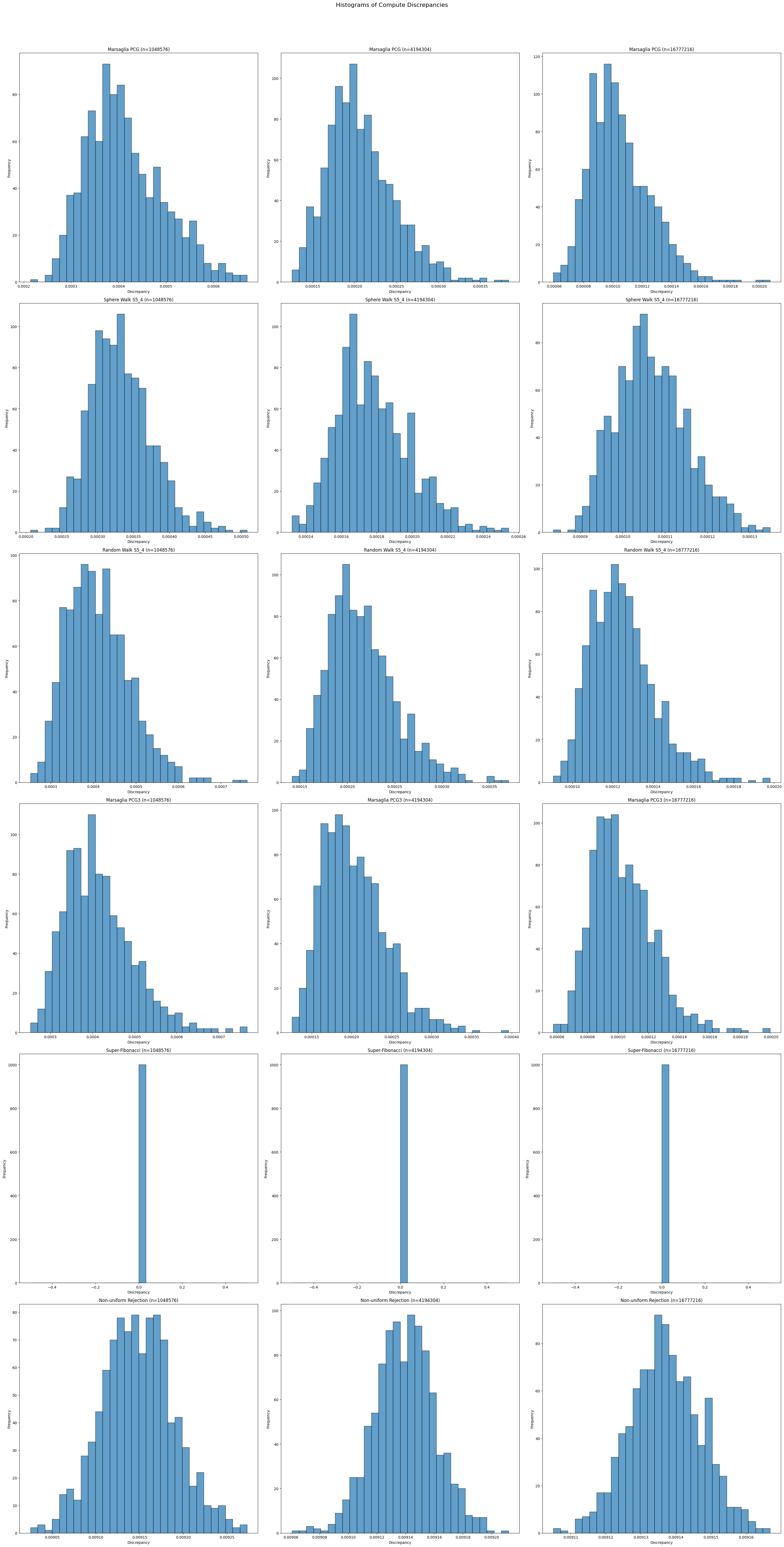
The fact that the rejection algorithm does not sample from the uniform distribution can be deduced by observing that the discrepancy stays constant as the point size goes up.
In contrast, the super Fibonacci algorithm is deterministic and therefore only appears as a Dirac measure.
In contrast to the xorshift and lcg random number generator which we used for the CPU implementation, we employed here recently discovered PCG variants.31
11. Normalization and using integers instead of floats
Quaternion multiplication will suffer from floating point drift. It is therefore required to normalize the internal state, at least every few ten thousand calls:
state = normalize(state);Since we are dealing with integer quaternions that are normalized, we may try to make the quaternion multiplication over the integers, doing the norm calculation separately. Of course, we expect an overflow after
quatz s5i[6] =
{
  1+2i, 1+2j, 1+2k, 1-2i, 1-2j, 1-2k
};

template <class RandomWalk>
quat sampler_quaternion_int_5()
{
	static RandomWalk walk{};
	static quatz q{};
	static u32 tt = 26;
	static u64 norm = 1;
	if (tt == 0)
	{
		q = {};
		tt = 26;
		norm = 1;
	}
	tt--;
	q = s5i[walk()] * q;
	norm2 *= 5u;
	return to_quat_f32(q, (f32)(1./std::sqrt(static_cast<f64>(norm2))));
}
Restarting the walk every
Consequentially, the first level
This implementation is twice as fast as its scalar version. But it is important to note that the discrepancy will not go below a certain threshold because of the error of short paths just addressed. Hence, it is only suitable for a small number of samples.
We can combine different Hecke operators
Source code for this project can be found on https://github.com/reneruhr/quaternions. It contains four programs (render , discrepancy, compute, compute_vk) that compile on Microsoft’s C++ compiler and a python script for plotting the graphs.
- Graphic Gems III, Shoemake. urot.c ↩︎
- Wiki reference. ↩︎
- https://en.wikipedia.org/wiki/Triple_product#Vector_triple_product ↩︎
- https://community.khronos.org/t/quaternion-functions-for-glsl/50140 ↩︎
- The construction of such measures for Lie groups is due to Hurwitz https://eudml.org/doc/58378 but they are now named after Haar who generalized the constructed to topological groups in https://doi.org/10.2307/1968346. (Links shared only for historic curiosity.) ↩︎
- Correct is any measurable set on which
μ ’s domain is restricted to exclude certain paradoxical properties as a later footnote shows. ↩︎ - http://www.graphicsgems.org/ ↩︎
- As observed in Graphics Gems III, the algorithm in Graphics Gems II, Section VII.7 does not sample the uniform measure. ↩︎
- A variant of this algorithm was recently studied in Sampling Rotation Groups by Successive Orthogonal Images ↩︎
- Choosing a Point from the Surface of a Sphere ↩︎
- Graphic Gems III, Shoemake. urot.c ↩︎
- See Hurwitz’ lecture notes Vorlesungen über die Zahlentheorie der Quaternionen on integer quaternions which are quite accessible. ↩︎
- A construction of Banach and Tarski uses the free group for a seemingly paradoxical reconstruction of sets. See Lubotzky’s book below. ↩︎
- Corollary 2.1.11 in Lubotzky’s book Discrete Groups, Expanding Graphs and Invariant Measures. ↩︎
- Hecke operators and distributing points on the sphere I and Hecke operators and distributing points on S2. II. See also these Bourbaki seminar notes for a concise summary. ↩︎
- Symmetric random walks on groups. There is no trivial eigenvalue
1 as with finite graphs. Kesten shows that 1 is contained in the spectrum of the averaging operator of a Cayley graph if and only if the group is amenable. ↩︎ - The first paper 8 actually only talks about the action of the rotation group on the 2-sphere. The book of Sarnak, Some Applications of Modular Forms discusses how to upgrade the result. The second paper 8 introduces the “Lattice method”, the approach taking by the book by Lubotzky which is extremely general, see e.g. Hecke operators and equidistribution of Hecke points.
↩︎ - Ellenberg, Michel, Venkatesh and a follow-up study on the large deviations principle in this situation by Khayutin ↩︎
- Breiman: The Strong Law of Large Numbers for a Class of Markov Chains
See also Section 3.2 Benoist, Quint: Random walks on reductive groups.
↩︎ - Chapter 3: Dolgopyat, Sarig: Local Limit Theorems for Inhomogeneous Markov Chains ↩︎
- See Spherical Fibonacci Point Sets for Illumination Integrals and a related book Efficient Quadrature Rules for Illumination Integrals references therein. The spherical Fibonacci point set seems to be the state of the art construction for low discrepancy point sets on the sphere. ↩︎
- Stolarsky, Theorem 2 in Sums of distances between points on a sphere. II. Formulas for the involved constants can be found in QMC designs: Optimal order Quasi Monte Carlo integration schemes on the sphere ↩︎
- Alexa: Super-Fibonacci Spirals: Fast, Low-Discrepancy Sampling of SO(3) ↩︎
- Section 3.3 Lecture notes of Sarig ↩︎
- Benoist and Quint Stationary measures and invariant subsets of homogeneous spaces (III) ↩︎
- Stackoverflow and Agner Fog: Extension to vector class library ↩︎
- https://mrelusive.com/publications/papers/SIMD-From-Quaternion-to-Matrix-and-Back.pdf ↩︎
- https://github.com/id-Software/DOOM-3-BFG/blob/1caba1979589971b5ed44e315d9ead30b278d8b4/neo/idlib/math/Simd_SSE.cpp ↩︎
- While the theorem13 of Benoist & Quint only holds for the simple, possibly biased, random walks, this paper generalizes some cases to the Markov chain situation required by the non-backtracking walk. Their setup does not cover the S-adic case but a generalization seems feasible. ↩︎
- https://www.techpowerup.com/gpu-specs/geforce-rtx-4070.c3924 ↩︎
- https://www.pcg-random.org/ and Hash Functions for GPU Rendering ↩︎


Leave a Reply