We introduce a new disk sampling algorithm that maps the square locally isometrically to the disk. Similar as to the classical rejection algorithm, this allows to push low discrepancy sampling strategies from the square to the disk with no warping. In contrast to rejection, it is amenable to SIMD implementations and our benchmark shows 2-3x performance increase on 256-bit width vectors.
First recall rejection sampling, in which the square circumscribing the disk is sampled and a sample may be rejected if it lies outside the disk.
point_2d rejection_sampling()
{
   f32 x,y;
   do
   {
      x = random_float(-1,1);
      y = random_float(-1,1);
   }
   while(x*x + y*y > 1);
   return {x,y};
}
In this post we modify this algorithm. We will sample the square inside the disk, so we will never reject any sample. To make up for the parts that we miss, we make use of some symmetries explained next.
\( \def\H{\mathbb{H}} \def\H1{\mathbb{H}^1} \def\N{\mathbb{N}} \def\E{\mathbb{E}} \def\Z{\mathbb{Z}} \def\R{\mathbb{R}} \def\C{\mathbb{C}} \def\S{\mathbb{S}} \def\V{\mathbb{V}} \def\HR{\H(\R)} \def\HU{\mathbb{H}^1(\mathbb{R})} \def\SU{\text{SU}(2)} \def\su{\mathfrak{su}_2} \def\SO{\text{SO}(3)} \def\So{\text{SO}(2)} \)The algorithm
We now present a new algorithm in which the rejection is replaced by “adoption”.
We introduce some notation:
- \(D = \{ p: \|p\|<=1 \}\) unit disk
- \(S = \{ (x,y) : |x|, |y|<=\sqrt{2} \}\) square inscribed in the unit disk
- \( H_1 = \{ (x,y) : x>0 \}, H_2 = \{ (x,y) : y>0 \}, H_3 = \{ (x,y) : x<0 \}, H_4 = \{ (x,y) : y<0 \} \) halfplanes
- \(⌓^D_{i} = \{ p\in D\cap H_i \setminus S \}\)
- \( t_1 = (-\sqrt{2},0), t_2 = (0,-\sqrt{2}), t_3 = (\sqrt{2},0), t_4 = (0,\sqrt{2}) \) translation vectors
- \(D_i = D+t_i = \{ p: \|p-t_i\|<=1 \}\) translated unit disks
- \(⌓^S_{i} = ⌓^D_{i} + t_i = S\cap D_{i}\)
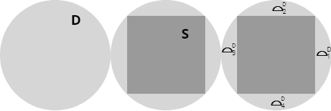


We sample from the square S inscribed in the unit disk D. We divide the points inside the disk that lie outside the square into four circular segments \(⌓^D_i\) of the initial disk D.
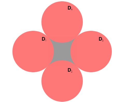
Consider further the 4 unit disks \(D_i\) centered at an offset of \(\pm\sqrt{2}\) on the horizontal and vertical axis. These disks intersect S in a 4 circular segments \(⌓^S_i\). We can choose the labeling of \(⌓^D_i\) and \(⌓^S_i\) such that \(⌓^D_i = ⌓^S_i\pm\sqrt{2}\) where translation is in the horizontal axis for odd i and vertical for even i. The sign is uniquely defined by i. For each point p in some \(⌓^S_i\), we let p’ its image in \(⌓^D_i\) by translating it by \(\pm\sqrt{2}\). This is the “adopted” point.
The sample strategy is now as follows:
- Let p be a uniform sample on S.
- Check if p lies in any of the \(D_i\).
- If not, take the sample p.
- If yes, then p is also inside some \(⌓^S_i\).
- Take the sample p, but also cache p’.
- In the next function call, we directly return p’.
Implementation
We now present a C++-like implementation. We scale the above described picture by \(\sqrt{2}\) so that the square \(S\) becomes the standard square of side length 2, and the final sample is inside disk of radius \(\sqrt{2}\), which we scale down by \(1/\sqrt{2} = \sqrt{2}/2\) before returning.
point_2d adoption_sampling()
{
   const f32 s2 = std::sqrt(2.f)/2;
   f32 x,y;
   static f32 x_cache = 0;
   static f32 y_cache = 0;

   if(x_cache != 0 || y_cache != 0)
   {
       x = x_cache;
       y = y_cache;
       x_cache = 0;
       y_cache = 0;
       return {s2*x,s2*y};
   }


   x_cache = x = random_float(-1,1);
   y_cache = y = random_float(-1,1);

   f32 r2 = x * x + y * y;
   f32 t = r2 + 2;

   if (t <= 4 * x)
   {
	x_cache -= 2;
   }
   else if (t <= -4 * x)
   {
	x_cache += 2;
   }
   else if (t <= 4 * y)
   {
	y_cache -= 2;
   }
   else if (t <= -4 * y)
   {
	y_cache += 2;
   }
   else
   {
      x_cache = y_cache = 0;
   }
   return {s2*x,s2*y};
}
Comparison with Rejection
We point out the differences to the rejection sampling strategy:
| Adoption | Rejection | |
| Sample multiplier | 1/(2-\(\pi/2\)) | \(\pi/4\) |
| Maximal instruction cost | 2 rng calls & 4 comparisons | \(\infty\) |
| Memory requirement | rng seed & last adopted sample | rng seed |
| Invertibility | with extra encoding | right inverse |
| Continuity | discontinuous at boundary of C | continous |
| Isometry | locally isometric | isometric |
| Symmetries | .73 probability of translational symmetry | none |
Sample multiplier
To produce n samples, the main body (producing random numbers and checking intersections) in the rejection algorithm has to run \(4/\pi n\) times in expectation. In the adoption algorithm, the main body only runs \( (2-\pi/2)n\) times on average. If the rng (random number generator) is expensive, say, because it is a custom low discrepancy sequence, then adoption is \(3 \approx \frac{4/\pi}{2-\pi/2}\) times as economic compared to rejection in expectation.
Maximal instruction cost
In the rejection algorithm, bad luck can cause many loop iterations. Of course, to run the main body of the rejection algorithm n-times decreases exponentially so that the expected iteration number equals one over the sample multiplier. The adoption cost in comparison has a fixed upper bound. This helps with SIMD implementation.
Memory requirement
The main disadvantage of the adoption strategy is that it needs memory. This makes GPU implementations more restrictive as invocations are not independent of each other.
Invertibility
Both strategies are not trivially invertible if one tries to reinterpret them as maps from a square to the disk. Rejection, can be understood as restriction map from square to disk, does have a right inverse, namely the inclusion map from disk to square.
Adoption can be understood as one-to-many mapping. It is possible to encode in each sample if it was adopted or not, which can be used to recover the original point from the square. This will be a many-to-one mapping.
Suppose we wish to use the inverse map to find a pixel from a square texture. For the rejection map, pixels outside the disk would simply be not used.
For the adoption map, values in the segments \(⌓^S_i\) will have to be compressed as they will hold two values, one for the point in \(⌓^S_i\) itself and one for the adopted copy in \(⌓^D_i\).
Continuity/Isometry
Inside the (open) disk, the rejection sample algorithm is continuous, since it is essentially the identity map. The adoption algorithm produces additional samples outside the set C, and points may suddenly disappear if they are move from outside C to inside C.
Symmetry
The adoption method makes use of antithetic variates, see the corresponding subsection below.
Markov Chain description
This algorithm describes a Markov chain on D as follows.
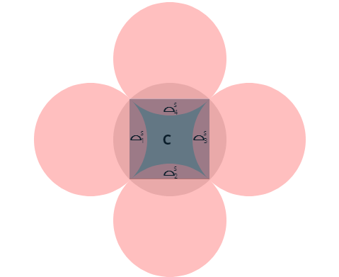
Let C be the complement of the \(⌓^S_i\) inside S.
For simplicity, label all the partition elements \(C, ⌓^S_1,⌓^S_2,⌓^S_3,⌓^S_4, ⌓^D_1, ⌓^D_2, ⌓^D_3, ⌓^D_4\) by \(P_i\).
Let \(m_i\) be the uniform measure on \(P_i\). Let m be the uniform measure on D.
The transition probability \(\rho(dx,y)\) of \(x\) given \(y\) (for each fixed y this is a measure) is easily seen to be \(\rho(dx,y) = m_{i_y}(dx) p_{i_x,i_y}\) where \(i_y,i_x\) are the indices for which \(y\in P_{i_y}, x\in P_{i_x}\) and \(p_{i_x,i_y}\) is the transition probability of a finite Markov chain on 9 symbols. Let \(m(⌓)\) denote the area of any of the circular segments.
Let \(a = m(⌓)/m(S)\) and note \( 1-4a = \frac{m(S)-4m(⌓)}{m(S)} = \frac{1-8m(⌓)}{m(S)} = m(C)/m(S). \)
Then
$$P=(p_{ji}) = \left[\begin{matrix} 1-4a & a & a & a & a & 0 & 0 & 0 & 0\\ 0 & 0 & 0 & 0 & 0 & 1 & 0 & 0 & 0\\ 0 & 0 & 0 & 0 & 0 & 0 & 1 & 0 & 0\\ 0 & 0 & 0 & 0 & 0 & 0 & 0 & 1 & 0\\ 0 & 0 & 0 & 0 & 0 & 0 & 0 & 0 & 1\\1-4a & a & a & a & a & 0 & 0 & 0 & 0\\1-4a & a & a & a & a & 0 & 0 & 0 & 0\\1-4a & a & a & a & a & 0 & 0 & 0 & 0\\1-4a & a & a & a & a & 0 & 0 & 0 & 0\end{matrix}\right]. $$
Solving \(\pi P = \pi\), we find the stationary distribution
$$\pi = (m(C), m(⌓),m(⌓),m(⌓),m(⌓),m(⌓),m(⌓),m(⌓),m(⌓)).$$
This chain is ergodic, and we can deduce convergence from that fact: Let \( x_i\) denote the outcomes of the sampling and let \(f:D\to\R\). We need to show that, almost surely,
$$\frac{1}{n}\sum_{i<n} f(x_i) \to m(f).$$ Reorder the sum according to which \(D_j\) each \(x_i\) falls into. Relabel them \(x_{j_k}\) and let \(n_j\) be their cardinalities:
$$\frac{1}{n}\sum_{i<n} f(x_i) = \sum_j\frac{n_j}{n} \frac{1}{n_j}\sum_{k<n_j} f(x_{j_k})$$
For each fixed j, the sequence \(x_{j_k}\) are sampled from \(m_j\). By the the law of large numbers for iid random variables1, \(\frac{1}{n_j}\sum_{k<n_j} f(x_{j_k})=m_j(f) + o(1)\) as \(n_j\to\infty\). By the ergodic theorem for Markov chains2, \(\frac{n_j}{n}= \pi_j + o(1)\) (in particularly, \(n_j\to\infty\)). Combining these two facts,
$$\frac{1}{n}\sum_{i<n} f(x_i) = \sum_j \pi_j m_j(f) + o(1) = m(f) + o(1).$$
Usage as warp function
Here we wish to study the use of the rejection and adoption sampler as warp functions in the following sense.
Suppose we have high quality low discrepancy point sets (qmc) on the square and we wish to map them to the unit disk. The two common strategies are the polar map and the concentric map3. See the Pixar Technical Memo4 on sampling which brings up this strategy or the PBRT book5.
Here we make the explicit case of using rejection and the adoption map, by replacing the uniform sampler by a qmc.
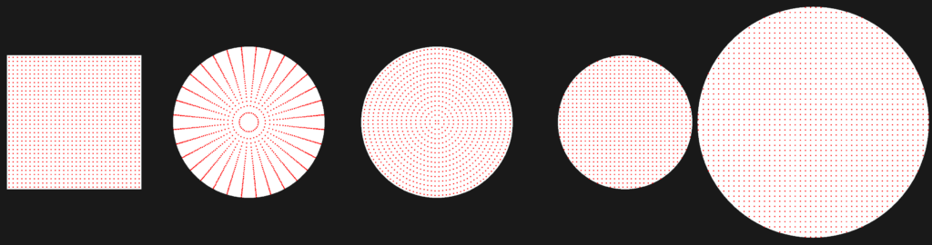
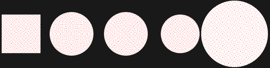
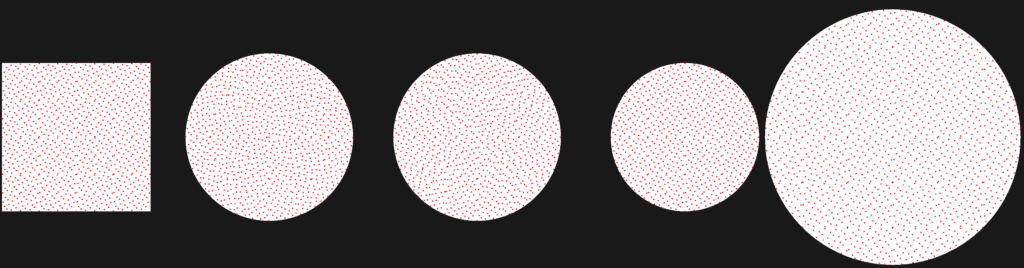
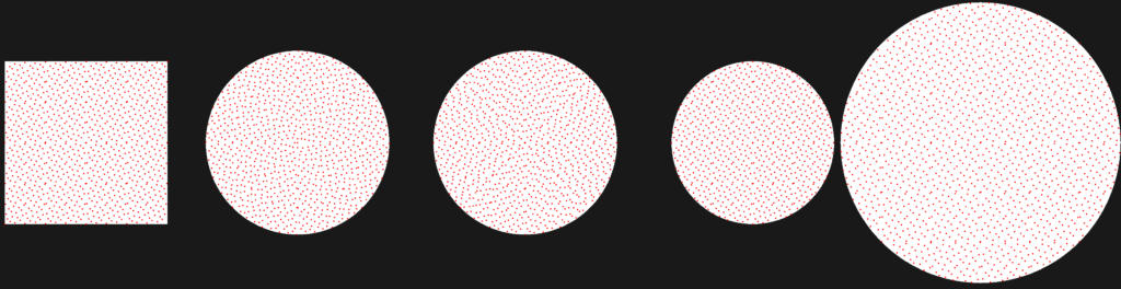
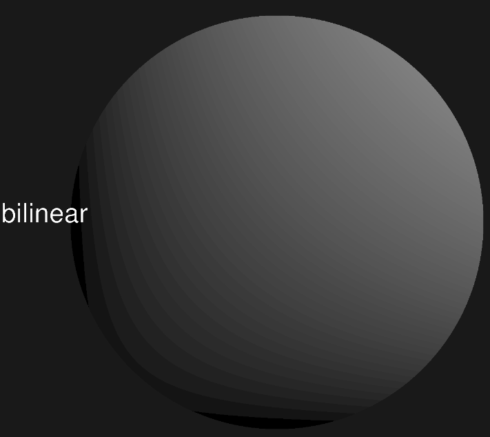
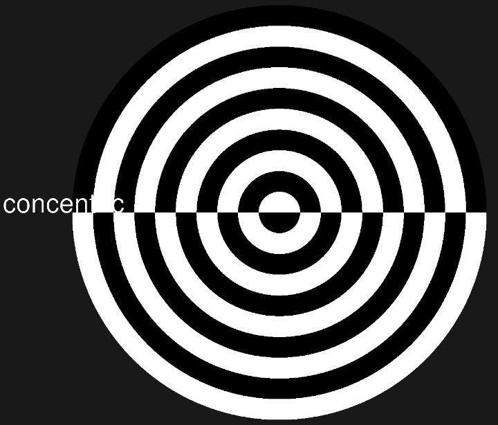
Some plots of qmc sequences on the square and their mappings on the disk using the four warps polar/concentric/rejection/adoption are shown next. The qmc sequences are taken from the Sampling and Reconstruction chapter of PBRT 4.
We plot the size of the disk according average number of samples produced per point on the square, which is one for polar/concentric, >1 for adoption and <1 for rejection.
Note how sets which exhibit the symmetries of a torus like the grid or the Sobol sequence feature seamless boarders around the square in the adoption method.
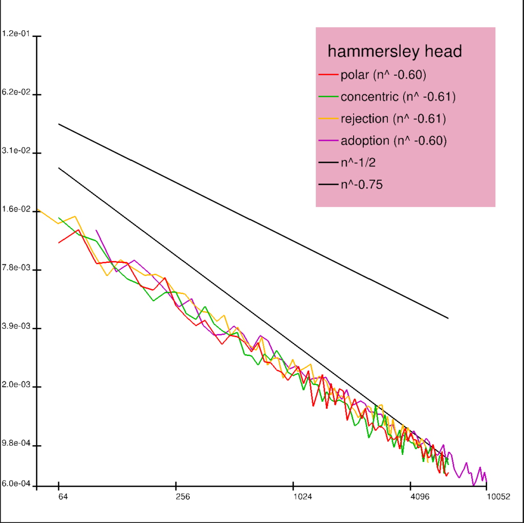
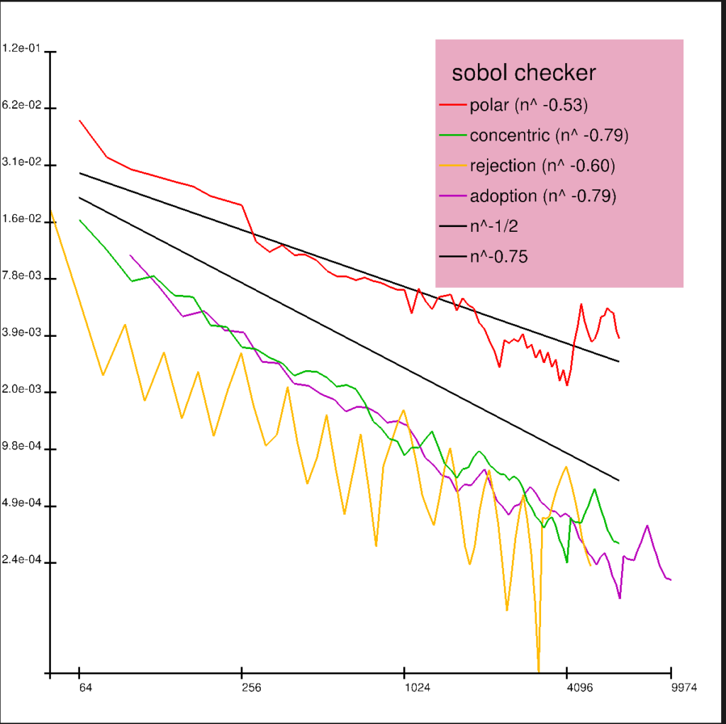
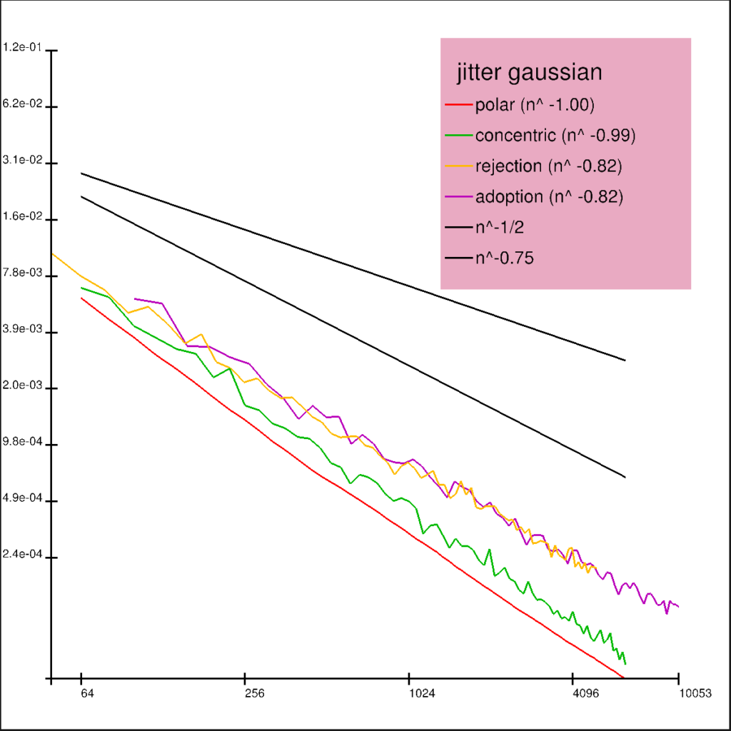
We show some discrepancy plots showing mean squared error of 100 trials against the total number of samples. The qmc methods are randomized using Owen scrambling6. Random refers to the uniform sampler, and jitter refers to the stratified sampler.

Antithetic variates
The notion antithetic variates8 refers to introducing area-preserving transformations which are applied to the sampled points. The standard example being negation on the real line or reflection around the origin inside the disk9. These can lead to lowered variance for odd functions, \(f(-x)=-f(x)\) but make sampling for even functions less effective. The other property was listed as a feature in the comparison table between adoption and rejection: An expensive sample might be made more economic if the symmetries are cheap to produce.
One may consider the adoption method to be a simple antithetic version of the restriction method. Indeed, given any rational rotation R of order n, one can generate additional (n-1) antithetic samples \(R^kx\) given some sampled point x on the circle of radius |x|.
In the method proposed here, antithetics are only produced on a subset of the disk, namely on the inner segments \(⌓^S_{i}\) and the transformations are translations \(T_i:⌓^S_{i}\to ⌓^D_{i}\).
The set C, which consists of the disk minus the eight segments ⌓ has relative area \(\frac{4}{\pi}-1\approx0.27\). This “pure” area is untouched by symmetries artificially introduced. If disk sampling is applied to cosine-weighted hemisphere sampling10, then the projection of C, also of relative area 0.27, is located around the north pole.
SIMD benchmarks
We now show performance characteristics of a SIMD implementation using AVX2 and AVX512. We produce 2^23=8388608 samples and do an discrepancy test against a collection of sets on the unit disk. The units in the following table are cycles per sample.
| AMD Zen 4 | AVX2 msvc | AVX2 clang | AVX512 msvc | AVX512 clang |
| polar | 4.65 | – | 3.16 | – |
| rejection | 7.99 | 7.76 | 5.50 | 5.32 |
| adoption | 3.61 | 2.67 | 3.94 (?!) | 2.06 |
Note that we did not succeed in getting the performance benefits AVX512 promises over AVX2, in fact we are slower using the msvc compiler. The mechanism for comparison in AVX512 uses mask vectors, forcing a different implementation which may causes the performance catastrophe.
We only found Intel’s SMVL library working for msvc which provides the sincos implementation, hence the polar version lacks from the profiling data for clang.
The associated github folder https://github.com/reneruhr/adoption for this project contains three programs: The animation video is a recording from an OpenGL program. The plots have also been drawn using OpenGL in a separate program. Finally, there is a test bench for the SIMD code. The programs compile on Windows.
Update 14.04.2024:
Alias method and GPU implementation
As pointed out in discussion with Won in the comments, there is an alias sampling strategy that both removes the need for a cache (making it easy to implement on the GPU) and removes any unwelcomed translational symmetries.
We use a variant of the alias method11 as follows: Recall that we sample inside a square S, which is subdivided into C and complement. The probability of sampling inside C is \(\frac{m(C)}{m(S)}\). We modify this probability to be \(m(C)\) (recall the normalization \(m(D)=1\)) by attaching an alias on the set S, i.e. we sample again, with an alias probability p. This results in an equation for p:
$$ m(C) = \frac{m(C)}{m(S)}(1-p) + \frac{m(C)}{m(S)}p\frac{m(C)}{m(S)}$$
which gives \(p =\frac{2}{\pi} (=m(S))\).
Having the correct probability for C, we sample inside \(⌓^S_i\) twice as often. We add an alias to \(⌓^D_i\) with alias probability 1/2.
Here’s a Cuda C++ implementation:
__global__ void adoption_sampling(vec2* out, u32 n)
{
    u32 idx = blockIdx.x * blockDim.x + threadIdx.x;
    if (idx < n)
    {
        u32 s = idx;
        f32 x,y;
        x = (s=rng(s)) * 0x1.0p-31f - 1.f;
        y = (s=rng(s)) * 0x1.0p-31f - 1.f;

	f32 r2 = x * x + y * y;
	f32 t = r2 + 2.f;
	f32 x_cache = x;
	f32 y_cache = y;

	if (t <= 4 * x)
	{
		x_cache -= 2;
	}
	else if (t <= -4 * x)
	{
		x_cache += 2;
	}
	else if (t <= 4 * y)
	{
		y_cache -= 2;
	}
	else if (t <= -4 * y)
	{
		y_cache += 2;
	}
        else
        {
           if((s=rng(s)) * 0x1.0p-32f < CUDART_2_OVER_PI_F)
           {
                x = (s=rng(s)) * 0x1.0p-31f - 1.f;
                y = (s=rng(s)) * 0x1.0p-31f - 1.f;

                r2 = x * x + y * y;
                t = r2 + 2.f;
                x_cache = x;
                y_cache = y;

                if (t <= 4 * x)
                {
                    x_cache -= 2;
                }
                else if (t <= -4 * x)
                {
                    x_cache += 2;
                }
                else if (t <= 4 * y)
                {
                    y_cache -= 2;
                }
                else if (t <= -4 * y)
                {
                    y_cache += 2;
                }
            }
        }

        if((s=rng(s)) < 1u<<31)
        {
            x_cache = x;
            y_cache = y;
        }

        out[idx].x = x_cache;
        out[idx].y = y_cache;

}
It is possible to optimize somewhat by directly checking if a point (x,y) is inside C using
bool inside_c = t > 4*fmaxf(fabsf(x),fabsf(y));
When comparing to the polar method, on a RTX 4070, it is clearly slower and at best comparable to rejection:
| ns/sample | |
| Polar | 0.0020 |
| Rejection | 0.0058 |
| Adoption | 0.0065 |
The algorithms are iterated 100 times inside the kernel calls to make the computational time dominate over the memory write times. Times are averages over 30 tries. The Cuda compile flag –use_fast_math for fast sin/cos is used.
The full code can be found in the Cuda folder on github.
- https://en.wikipedia.org/wiki/Law_of_large_numbers ↩︎
- https://en.wikipedia.org/wiki/Discrete-time_Markov_chain ↩︎
- Shirley & Chiu: A Low Distortion Map Between Disk and Square ↩︎
- Andrew Kensler: Correlated Multi-Jittered Sampling ↩︎
- PBRT 4: A.5.1 Sampling a Unit Disk ↩︎
- PBRT 4: util/lowdiscrepancy.h ↩︎
- PBRT 4: Sobol Sampling ↩︎
- https://en.wikipedia.org/wiki/Antithetic_variates ↩︎
- Fishman & Huang: Antithetic variates revisited ↩︎
- PBRT 4: Hemisphere Sampling ↩︎
- PBRT 4: A.1 The Alias Method ↩︎
Leave a Reply